For Numerical Simulations Supported by Database in Fortran

Author: Amasaki Shinobu (雨崎しのぶ)

Posted on: 2023-12-02 JST

Abstract

I previously have posted an article titled ‘Accessing a Database Server via Fortran.’ In this article, I would like to continue from that point, and illustrate how to manage data in a numerical computing program using Libpq-Fortran and PostgreSQL.

Introduction
Example Problem: 1-D Advection Equation
Preparation
Execute Simulations
Retrieve the Data for Plot
Conclusion

Introduction

The primary goal for many Fortran programmers is likely to write numerical computing programs and evaluate thier results. Here, the process of numerical simulation can be classified as follows:

Write the source code on source files.
Execute the simulation by providing input files and obtain output files.
Visualize the results using a plotting script and obtain image files.
goto 1 (Repeat the process by returning to step 1).

When it comes to managing these files, it is generally evident that utilizing a version control system (e. g. Git, SVN) is the best approach for handling source code and scripts that are constantly changing. On the other hand, determining the most effective method for managing input and output files in Step 2 is not as straightforward.

If opting for file system management, one might attempt the following naming and directory structuring:

Assign unique names by adding timestamps or keywords to the file names, such as foobar_20231210_123456_baz.dat.
Use directories for categorization, for instance, result/foo-scheme/bar-simulation/baz_20231210.dat

These methods can encounter issues such as name collisions when parallel processing, longer directory paths leading to increased complexity in extracting data, and the inconvinience of devising lengthly unique names. Dealing with these problems, while manageable manually for a small amount of data, may become impractical as the data volume increases substantially.

In this article, we will discuss practical methods for managing the continuously increasing data from numerical simulaitons using PostgreSQL—a relational database management system— and Libpq-Fortran—its Fortran frontend.

Example Problem: 1-D Advection Equation

Taking the numerical simulation of the one-dimensional advection equation as an example, we vary parameters, execute simulaitons, and register the results in a database.

The one-dimensional advection equation is given by:

\[\frac{\partial u}{\partial t} + \frac{\partial f}{\partial x} = 0, f= cu.\]

Discretizing this equation using the explicit Eular method, Lax-Friedrich scheme and Lax-Wendroff scheme, we obtain the following difference equations:

Explicit Eular method:

\[ u^{n+1}_{j} = u^{n}_{j} - \frac{\Delta t}{\Delta x} ( \tilde f^{n+\frac{1}{2}}_{j+\frac{1}{2}} - \tilde f^{n-\frac{1}{2}}_{j-\frac{1}{2}}),\]

Lax-Friedrich scheme:

\[\tilde f ^{n+\frac{1}{2}}_{j+\frac{1}{2}} = \frac{1}{2}[(f^n_{j+1} + f^n_j) - \frac{\Delta x}{\Delta t}(u^n_{j+1} - u^n_j)],\]

Lax-Wendroff scheme:

\[\tilde f ^{n+\frac{1}{2}}_{j+\frac{1}{2}} = \frac{1}{2}[(1 - c\frac{\Delta t}{\Delta x})f^n_{j+1}+ (1+ c\frac{\Delta t}{\Delta x})f^n_j], \]

where \(\tilde f\) is the numerical flux, \(f^n_{j} = f(u^n_j) = cu^n_j\), \(c\) represents the characteristic speed, \(\Delta t\) is the time step size, and \(\Delta x\) is the spatial grid spacing.

The three quantities, \(c\), \(\Delta t\), and \(\Delta x\), characterize a simulation of this equation, serving as parameters that defines a single simulation.

Preparation

Create User and Database

In the following Fortran program, it connect to a PostgreSQL server on the localhost and executes two commands.

program create_database
   use, intrinsic :: iso_c_binding
   use :: libpq
   implicit none
   
   type(c_ptr) :: conn, res
   character(:), allocatable :: conninfo, query
   
   conninfo = "host=localhost user=postgres"
   
   ! Connect
   conn = PQconnectdb(conninfo)
   
   ! Error handling for connection 
   if (PQstatus(conn) /= CONNECTION_OK) then
      print *, PQerrorMessage(conn)
      error stop
   end if

   ! Command to create a user account
   query = "create role shinobu with createdb login password 'foobar';"
   res = PQexec(conn, query)

   ! Error handling for command execution
   if (PQresultStatus(res) /= PGRES_COMMAND_OK ) then
      print *, PQresultErrorMessage(res)
      call PQfinish(conn)
      error stop
   end if

   call PQclear(res)

   ! Command to create database 'simulation'
   query = "create database simulation with owner shinobu;"
   res = PQexec(conn, query)

   ! Error handling for command execution 
   if (PQresultStatus(res) /= PGRES_COMMAND_OK ) then
      print *, PQresultErrorMessage(res)
   end if

　　! Free the result object
   call PQclear(res)
   
   ! Free the connection object
   call PQfinish(conn)

end program create_database

Here, feel free to modify the server address, create a username and password, and choose the database name according to your environment. Throughout this article, for example, we assume the server host is localhost, the username is shinobu, the password is foobar, and the database name is simulation. Note that at the initial connection, it connects to the PostgreSQL server on localhost with the administrator account postgres. If necessary, you should add password=password-of-postgres to the conninfo string.

Create Table

Next, we prepare a table to actually write simulation information.

Here, you need to use the user, database, and password created in the previous section for the connection information written in conninfo.

program create_table
   use :: libpq
   use, intrinsic :: iso_c_binding
   implicit none
   
   type(c_ptr) :: conn, res
   character(:), allocatable :: conninfo, query
   integer :: i

   conninfo = "host=localhost user=shinobu dbname=simulation password=foobar"
   conn = PQconnectdb(conninfo)
   if (PQstatus(conn) /= 0) then
      print *, PQerrorMessage(conn)
      error stop
   end if

   query = "create table advection &
   & (sim_id      decimal(4,0)      not null, &
   &  start_date  date              ,         &
   &  sim_name    varchar(100)      not null, &
   &  cs          double precision  not null, &
   &  dt          double precision  not null, &
   &  dx          double precision  not null, & 
   &  courant     double precision  ,         &
   &  length      double precision  ,         &
   &  nx          integer           not null, &
   &  nstep       integer           not null, &   
   &  dat_file    varchar(256)      not null, &
   &  primary key(sim_id));"
   
   res = PQexec(conn, query)
   if (PQresultStatus(res) /= PGRES_COMMAND_OK) then
      print *, PQresultErrorMessage(res)
   end if 

   call PQclear(res)
   call PQfinish(conn)

end program create_table

As indicated by the beginning of the string variable query with ‘create table advection’, this query creates a table named advection. This subsequent continuation lines list multiple attributes of the table, including their names, types, and options. And the primary key(sim_id) on the final continuation line specifies an attribute with a constraint to uniquely identify records in this table.

Check the Table

After running this program, you can inspect the database and table information using the psql command, which is PostgreSQL’s command-line interface.

Executing the command psql -h localhost -U shinobu -d simulation in the terminal and querying select * from advection; at the simulation=> prompt, if you obtain a list of attribute names like the following, it indicates success.

$ psql -h localhost -U shinobu -d simulation
psql (15.4)
Type "help" for help.

simulation=> select * from advection;
 sim_id | start_date |   sim_name    | cs |   dt   |  dx   | courant | l | nx  | nstep |      dat_file
--------+------------+---------------+----+--------+-------+---------+---+-----+-------+--------------------

We will proceed to register data for this table.

Execute Simulations

The program to be executed here consists of the following elements:

Main Program: With experiments for two different schemes, it has 2 loops that run 32 experiment in total, varying parameters for each experiment.
Internal procedures:
- main_loop subroutine: Takes parameters characterizing a simulation as arguments and executes single simulation.
- data_output subroutine: Writes values of x in the first columun and u in the second column to output file, with two empty lines as separators between data sets to facilitate reading reading by Gnuplot.
- data_registration subroutine: After the execution of main_loop, registers the experiment parameters and the path to the output file in the database.

`main_loop`

The time integration loop for numerical simulation is included in the main_loop subroutine. This subroutine takes parameters characterizing one experiment as arguments. When this subroutine is executed, the filename is stored in the argument filename, and the experiment result are written to a .dat file with this name.

subroutine main_loop(cs, dt, dx, nstep, filename, offset_k, k, prefix)
   implicit none
   real(real64), intent(in) :: cs, dt, dx
   integer(int32), intent(in) :: k
   character(:), allocatable, intent(inout) :: filename
   integer :: offset_k
   character(*), intent(in) :: prefix
   integer, intent(out) :: nstep

   character(4) :: code
   integer :: nth_out
   real(real64) :: tout, time
   real(real64) :: Courant

   integer :: i
   integer :: uni

   real(real64), allocatable :: x(:)
   real(real64), allocatable :: u(:), f(:), u_new(:), f0(:)

   write(code, '(1i4.4)') k + (offset_k - 1)

   Courant = cs*dt/dx

   write(error_unit, '(a, i0, a)') "### START ", k, "-th Simulation ###"
   write(error_unit, '(a, f10.3)') " Courant number: ", Courant

   ! Initialize
   uni = 100
   nth_out = 0
   nstep = 1
   time = 0d0
   tout = 0
   allocate(x(0:nx), source=0d0)
   allocate(u(0:nx), source=0d0)
   allocate(u_new(0:nx), source=0d0)
   allocate(f0(0:nx), source=0d0)
   allocate(f(0:nx), source=0d0)
   
   ! set spacial grid
   x(0) = 0d0
   do i = 1, nx
      x(i) = x(0) + dx*dble(i)
   end do

   ! Initial condition
   do i = 0, nx
      if (x(i) < 0.1d0) then
         u(i) = 1d0
      else
         u(i) = 0d0
      end if
   end do

   filename = 'result/'//trim(adjustl(prefix))//code//'.dat'
   
   open(uni, file=filename, form='formatted', status='replace')
   call data_output(uni, x, u, tout, time, 0, nth_out)

   ! time integration loop
   do
      nstep = nstep + 1
      time = time + dt

      f0(:) = cs*u(:) ! numerical flux

      ! Lax-Friedrich scheme
      if (trim(prefix) == 'LF_') then
         do i = 1, nx-1
            f(i) = 0.5d0*(f0(i+1)+f0(i)) - 0.5d0*dx/dt *(u(i+1) - u(i))
         end do          
      end if

      ! Lax-Wendroff scheme
      if (trim(prefix) == 'LW_') then
         do i = 1, nx-1
            f(i) = 0.5d0*( (1d0-Courant)*f0(i+1) + (1d0+Courant)*f0(i) )
         end do
      end if

      ! Explicit Eular method
      do i = 1, nx-1 
         u_new(i) = u(i) - Courant*(f(i) - f(i-1))
      end do

      ! Update u
      u(2:nx-1) = u_new(2:nx-1)

      ! Boundary Condition
      u(1) = u(2)
      u(nx) = u(nx-1)

      if (time >= tout) call data_output(uni, x, u, tout, time, nstep, nth_out)
      if (time >  tend) exit

   end do

   close(uni)
   write(error_unit, fmtStop) nstep, time
   write(error_unit, '(a)') "### Normal STOP ###"
end subroutine main_loop

Within the included do-loop, the calculation of the numerical flux for the two schemes, as illustrated in the previous section’s mathematical expressions, is performed by switching based on the value of the argument prefix.

`data_output`

The subroutine for writing data is as follows:

subroutine data_output (uni, x, u, tout, time, nstep, nth_out)
   implicit none
   integer, intent(in) :: uni
   real(real64), intent(in) :: x(:), u(:)
   real(real64), intent(inout) :: tout
   real(real64), intent(in) :: time
   integer, intent(in) :: nstep
   integer, intent(inout) :: nth_out 
   integer :: i

   do i = 1, nx
      write(uni, fmtOut) x(i), u(i)
   end do
   
   ! Write two empty lines (for separating datasets for Gnuplot) into the file.
   write(uni, '(/)')  

   tout = tout + tout_interval
   
   write(error_unit, fmtErrOut) nstep, time, nth_out
   nth_out = nth_out + 1
end subroutine data_output

`data_registration`

The subroutine for registering data in the database is as follows:

subroutine data_registration(conn, simu_name, filename, offset_k, k, cs, dt, dx, nstep, date)
   use :: iso_c_binding
   use :: libpq
   implicit none
   type(c_ptr), intent(in) :: conn
   character(*), intent(in) :: simu_name
   character(*), intent(in) :: filename
   integer, intent(in) :: k, offset_k
   real(real64), intent(in) :: cs, dt, dx
   integer, intent(in) :: nstep
   character(*), intent(in) :: date

   character(:), allocatable :: query
   character(256) :: values(11)

   type(c_ptr) :: res
   real(real64) :: Courant
   character(4) :: code
   integer :: i

   Courant = cs*dt/dx

   ! Write the values into array 
   write(code, '(1i4.4)') k + (offset_k-1)
   values(1) = code
   values(2) = trim(adjustl(date))
   values(3) = trim(simu_name)
   write(values(4),  '(f16.8)') cs
   write(values(5),  '(f16.8)') dt
   write(values(6),  '(f16.8)') dx
   write(values(7),  '(f16.8)') Courant
   write(values(8),  '(f16.8)') L 
   write(values(9),  '(i0)') nx
   write(values(10), '(i0)') nstep
   values(11) = trim(adjustl(filename)) 

   do i = 1, size(values)
      values(i) = trim(adjustl(values(i)))
   end do

   query = 'insert into advection &
   &        (sim_id, start_date, sim_name, cs, dt, dx, courant, l, nx, nstep, dat_file) &
   & values ($1,     $2,         $3,       $4, $5, $6, $7,     $8, $9, $10,   $11)'

   res = PQexecParams(conn, query, size(values), [(0, i=1,size(values))], values(:))

   if (PQresultStatus(res) /= PGRES_COMMAND_OK) then
      print *, PQresultErrorMessage(res)
   end if

   call PQclear(res)

end subroutine data_registration

This includes a query called the insert statement, which inserts a record into the table in the database.

This insert statement is executed using the PQexecParams function, which allows you to include placeholders in the command string and pass their values separately as an array of strings. For detailed information about the arguments of this function, please refer to the PQexecParams page in the Libpq-Fortran documentation.

Execute Main Program

All necessary ingredients are now in place. Write the main program and execute the simulations. The entire code of main program can be obtained from this link on GitHub.

program main
   use, intrinsic :: iso_fortran_env
   use, intrinsic :: iso_c_binding
   use :: libpq

   implicit none

   real(real64), parameter :: tend = 0.6d0
   real(real64), parameter :: tout_interval = 0.1d0

   integer, parameter :: NX = 200     ! The number of spatial grid divisions 
   real(real64), parameter :: L = 1d0 ! The length of computing region 

   character(*), parameter  :: fmtOut   = '(e10.3, 1x, e10.3, 1x, i0)'
   character(*), parameter  :: fmtErrOut= "('  output  ', 'step=', i8, ' time=', e10.3, ' nth_out =', i3)"
   character(*), parameter  :: fmtStop  = "('  stop    ', 'step=', i8, ' time=', e10.3)"
   
   character(:), allocatable :: filename
   integer :: k

   real(real64) :: cs, dt, dx
   integer :: nstep, offset_k

   type(c_ptr) :: conn
   character(:), allocatable :: conninfo
   character(10) :: date = '2023-12-10'
   
   ! Connection
   conninfo = 'host=localhost dbname=simulation user=shinobu'
   conn = PQconnectdb(conninfo)

   if (PQstatus(conn) /= 0) then
      print *, PQerrorMessage(conn)
      error stop 
   end if

   ! Execute 16 simulations on Lax-Friedrich scheme (id = 1:16).
   offset_k = 1
   do k = 1, 16
      cs = 1d0
      dt = 5d-4  + 3d-4*dble(k-1)
      dx = L/dble(nx)
      call main_loop(cs, dt, dx, nstep, filename, offset_k, k, 'LF_')
      call data_registration(conn, 'Lax-Friedrich', filename, offset_k, k, cs, dt, dx, nstep, date)
   end do
   
   ! Execute 16 simulations on Lax-Wendroff scheme (id=17:32)
   offset_k = 17
   do k = 1, 16
   	cs = 1d0
   	dt = 5d-4  + 3d-4*dble(k-1)
   	dx = L/dble(nx)
   	call main_loop(cs, dt, dx, nstep, filename, offset_k, k, 'LW_')
      call data_registration(conn, 'Lax-Wendroff', filename, offset_k, k, cs, dt, dx, nstep, date)
   end do
   
contains

　! This includes the three subroutines mentioned above.
　! ...
　
end program main

Check the Registered Data

Execute psql -h localhost -U shinobu -d simulation in the terminal to launch psql, then run select * from advection; to confirm that 32 records have been inserted.

With this, we have successfully registered the result of numerical simulations into the database server. In the next section, we will demonstrate how to retrieve the registered data and draw plots from Fortran.

Retrieve the Data for Plot

Here, we will describe the process of retrieving data managed in PostgreSQL using Libpq-Fortran, passing the values from Fortran to a Gnuplot script, and drawing plots.

It is noting that if you wish to specify the drawing process in detail using Fortran, you may need to utilize libraries such as PLPlot.

The procedure here is as folllows:

Extract some records from the advection table in the simulation database.
Output the file paths of these data files.
Concatenate them into a string variable separated by spaces and pass it as command-line arguments to the script.

The following code is a sample program for plot.f90:

program plot
   use :: libpq
   use, intrinsic :: iso_c_binding
   implicit none
   
   character(:), allocatable :: conninfo, query, cmd
   type(c_ptr) :: conn, res
   integer :: i

   ! Connection
   conninfo = "host=localhost dbname=simulation user=shinobu"
   conn = PQconnectdb(conninfo)
   if (PQstatus(conn) /= 0) then
      print *, PQerrorMessage(conn)
      error stop
   end if

	cmd = "gnuplot -c plot.gp "

   query = "select dat_file from advection where sim_name = 'Lax-Wendroff' and courant > 0.55;"
   
   ! Execute the query
   res = PQexec(conn, query)

   ! Error Handling
   if (PQresultStatus(res) /= PGRES_COMMAND_OK) then
      print *, PQresultErrorMessage(res)
      call PQfinish(conn)
      error stop
   end if 

   ! Concatenate
   do i = 0, PQntuples(res) - 1
      cmd = cmd // ' '// PQgetvalue(res, i, 0)
   end do

   ! Execute the command
	print *, cmd
   call system(cmd)

   call PQclear(res)
   call PQfinish(conn)
   
end program plot

In this program, the query "select dat_file from advection where sim_name = 'Lax-Wendroff' and courant > 0.55;" instructs to extract and output file paths for all records where the simulation name is ‘Lax-Wendroff’ and the Courant number is greater than 0.55.

The results of this query are extracted from the object indicated by the c_ptr type variable res using functions provided by libpq. In the concatenation’s do loop, a loop is instructed to run for PQntuples(res) -1 iterations, starting from 0. Within this loop, the function PQgetvalue(res, i, 0) is called to retrieve the data from the i-th row and 0th column, and it is concatenated into the variable cmd.

The actual command to be executed would be as the following:

gnuplot -c plot.gp  result/LW_0024.dat result/LW_0025.dat result/LW_0026.dat result/LW_0027.dat result/LW_0028.dat result/LW_0029.dat result/LW_0030.dat result/LW_0031.dat result/LW_0032.dat

Here, plot.gp would be a Gnuplot script like the following:

set term pngcairo size 1600,1200
set termoption noenhanced
set output "plot9.png"

set xlabel "x"
set ylabel "u"
set xrange [0:1]
set yrange [-0.5:2.0]

set multiplot layout 3,3

do for [i=1:9] {
   path = ARGV[i]
   set title path

   unset xlabel
   unset ylabel
   if ( i % 3 == 1) {
      set ylabel "u"
   }
   if ( i > 6 ) {
      set xlabel "x"
   }

   plot  path index 0 using 1:2 with lines title 't = 0.0', \
      path index 1 using 1:2 with lines title 't = 0.1', \
      path index 2 using 1:2 with lines title 't = 0.2', \
      path index 3 using 1:2 with lines title 't = 0.3', \
      path index 4 using 1:2 with lines title 't = 0.4', \
      path index 5 using 1:2 with lines title 't = 0.5', \
      path index 6 using 1:2 with lines title 't = 0.6
}

unset multiplot

Please use the latest version of Gnuplot to execute this script.

Executing this program (plot.f90) allows you to generate an image like the following:

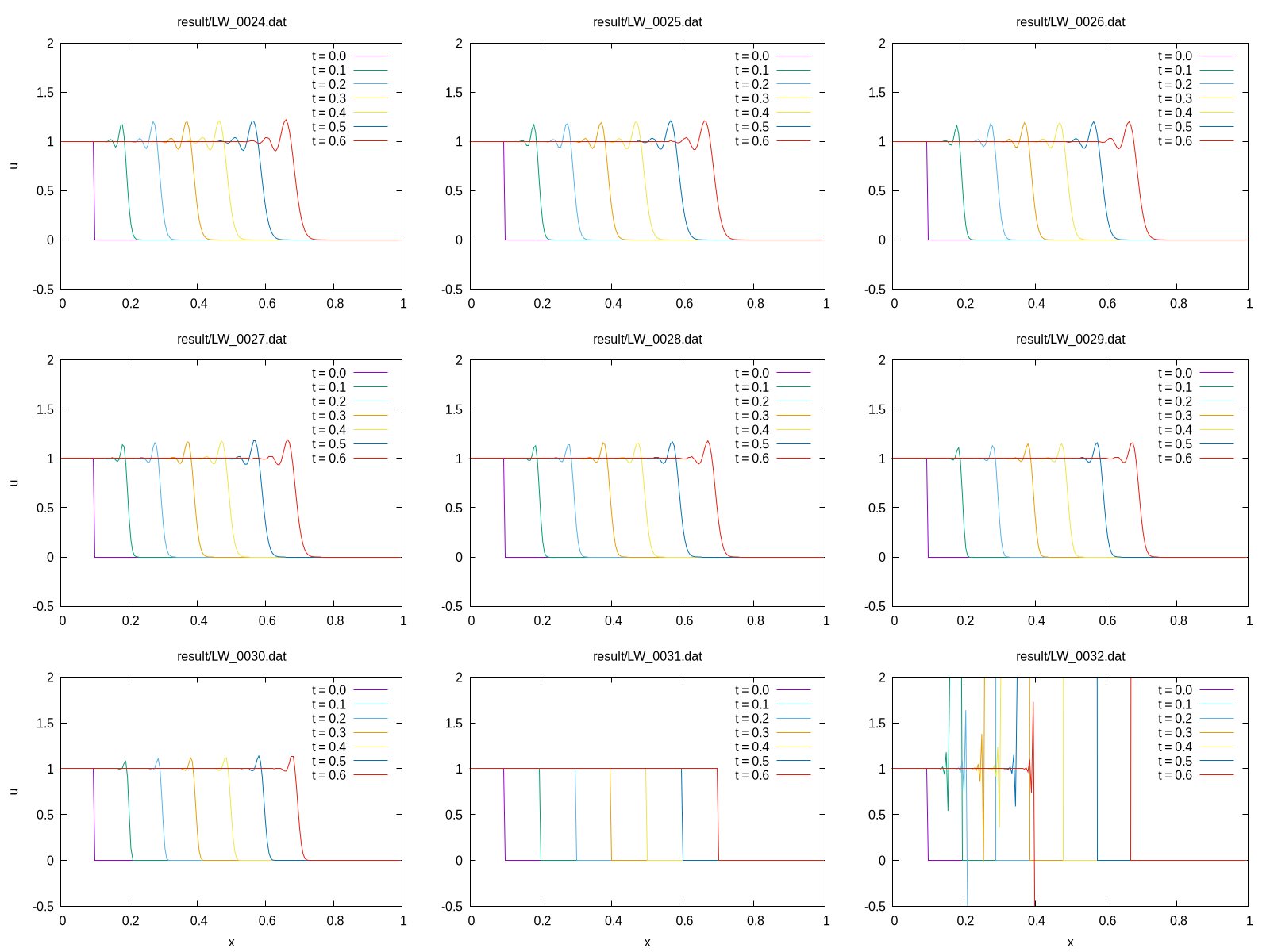
In conclusion, we have successfully loaded data from a PostgreSQL server using Libpq-Fortran and drawn a plot with a Gnuplot script.

Conclusion

I have described the process of registering numerical simulation data in PostgreSQL using the Libpq-Fortran library and retrieving that data from the server for further use.

This approach is obviously useful in scenarios where the same program needs to be executed massively with varying parameters. There have been instances when I chose to leverage a database for parameter exploration, particularly when conducting an exhaustive search of parameters to evaluate the stability of a finite difference scheme. As seen throughout this process, it’s now possible to directly register data from Fortran, whereas at that time, the data registration was done from another language.

In the example we covered this time, it was relatively easy to manage because one simulation corresponded to one record. However, if we consider cases where multiple files are output for a single simulation, the complexity of data management increases. I hope to write about this aspect at some point in the future.